人工智能（ArtificialIntelligence）

运行环境：MacBook Pro M1Max 32G 1T
本文主要以PyTorch为主

资源链接

环境安装

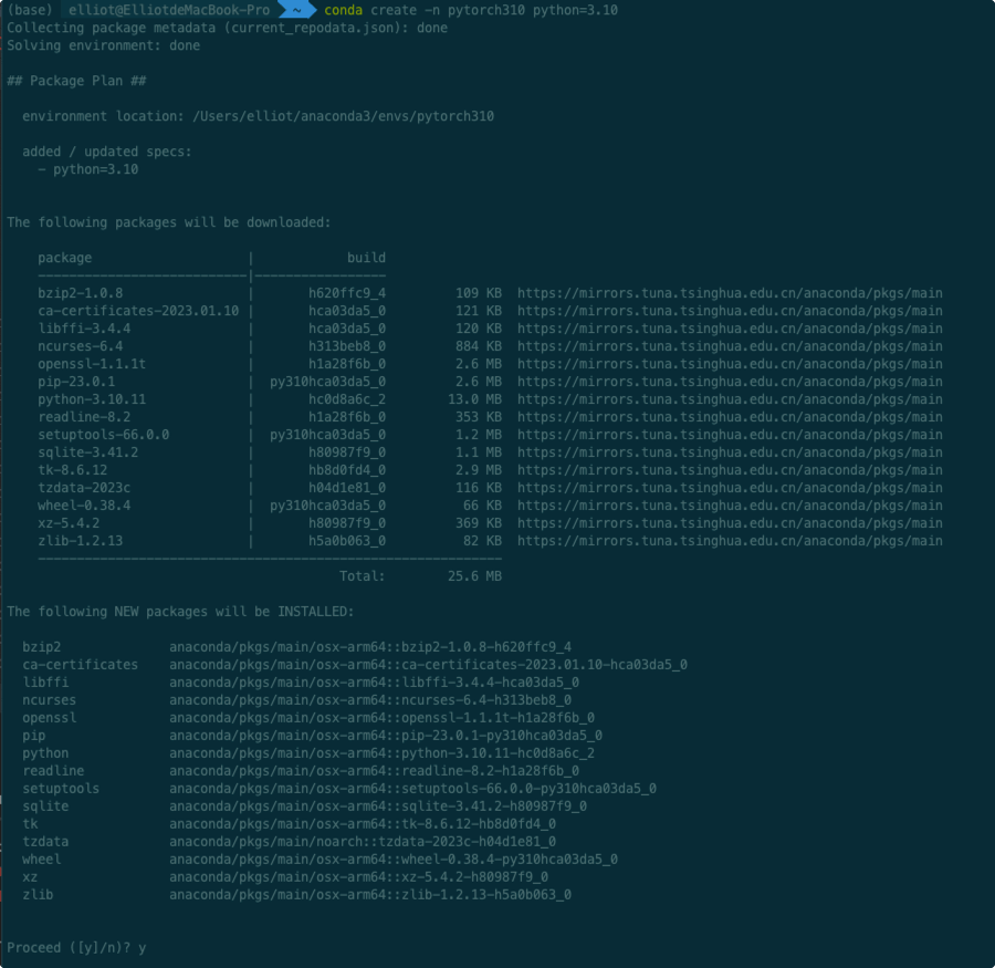
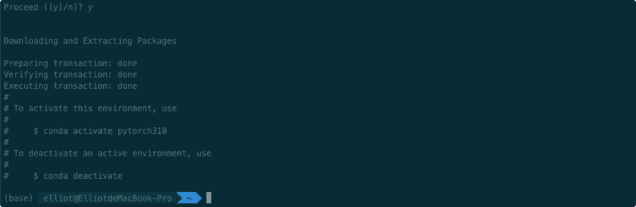
创建环境命令

conda create -n pytorch310 python=3.10

初始化界面激活环境命令

conda activate pytorch310

去激活环境命令

conda deactivate

报错处理：

1.移除代理
```
conda config --remove-key proxy
```
1

2.使用镜像

conda config --set remote_read_timeout_secs 600 conda config --add channels https://mirrors.tuna.tsinghua.edu.cn/anaconda/pkgs/free/
conda config --add channels https://mirrors.tuna.tsinghua.edu.cn/anaconda/pkgs/main/
conda config --add channels https://mirrors.tuna.tsinghua.edu.cn/anaconda/cloud/pytorch/

1
2
3

3.临时禁用代理

conda config --set proxy_servers.http ""
conda config --set proxy_servers.https ""

1
2

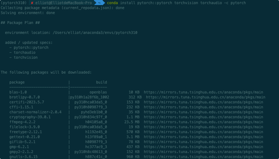
Pytorch安装 官网地址

选择对应的版本，复制命令即可

省略其余安装包

安装完成

验证是否安装成功

pip 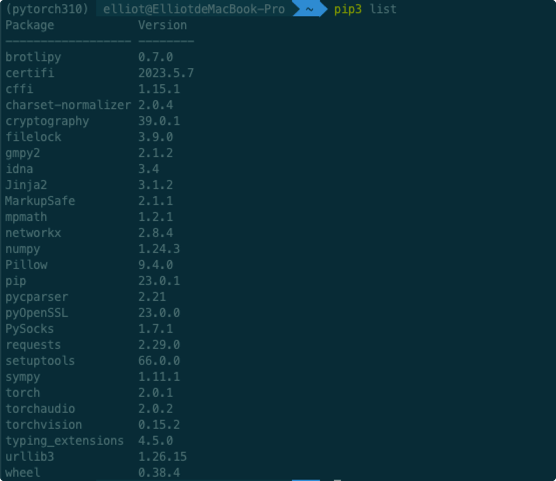验证是否安装成功

命令行导入测试，无报错则安装成功

！验证GPU加速

验证GPU加速

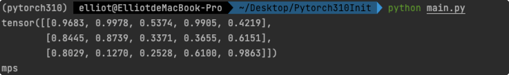
import torch
a = torch.rand(3,5)
print(a)
b = torch.device('mps')
print(b)

1
2
3
4
5

编辑器安装

Pycharm 下载地址

Jupiter 安装及使用

python < 3.10 以下可使用 conda install nb_conda

python >= 3.10 可使用 conda install -c conda-forge nb_conda_kernels

开启Jupyter NoteBook命令：jupyter notebook

激励函数 (Activation)

激励函数根据不同情况需要有不同选择

卷积神经网络：ReLU
循环神经网络：Relu Or Tanh

在AnaConda中使用matplotlib

conda install matplotlib

激励函数

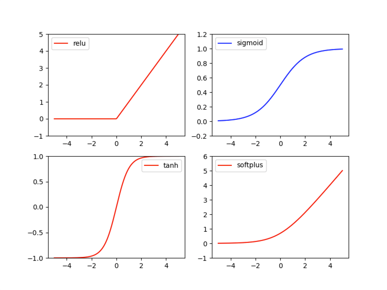
# 激励函数
import torch
import torch.nn.functional as F
from torch.autograd import Variable
import matplotlib.pyplot as plt

# fake data
# x data (tensor), shape=(100,1)
x = torch.linspace(-5, 5, 200)
x = Variable(x)
x_np = x.data.numpy()

y_relu = F.relu(x).data.numpy()
y_sigmoid = F.sigmoid(x).data.numpy()
y_tanh = F.tanh(x). data.numpy()
y_softplus = F.softplus(x).data.numpy()


plt.figure(1, figsize=(8, 6) )
plt.subplot(221)
plt.plot(x_np, y_relu, c='red', label='relu')
plt.ylim((-1, 5))
plt.legend(loc='best')

plt.subplot(222)
plt.plot(x_np, y_sigmoid, c='blue', label='sigmoid')
plt.ylim((-0.2, 1.2))
plt.legend(loc='best')


plt.subplot(223)
plt.plot(x_np, y_tanh, c='red', label='tanh')
plt.ylim((-1, 1))
plt.legend(loc='best')

plt.subplot(224)
plt.plot(x_np, y_softplus, c='red', label='softplus')
plt.ylim((-1, 6))
plt.legend(loc='best')

plt.show()

1
2
3
4
5
6
7
8
9
10
11
12
13
14
15
16
17
18
19
20
21
22
23
24
25
26
27
28
29
30
31
32
33
34
35
36
37
38
39
40
41

回归 Regression

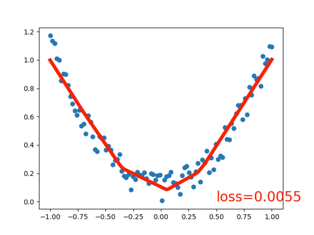
# 回归 Regression 

import torch
import torch.nn.functional as F
from torch.autograd import Variable
import matplotlib.pyplot as plt

x = torch.unsqueeze(torch.linspace(-1, 1, 100), dim=1)
y = x.pow(2) + 0.2 * torch.rand(x.size())

x, y = Variable(x), Variable(y)


# 打印
# plt.scatter(x.data.numpy(), y.data.numpy())
# plt.show()

class Net(torch.nn.Module):
    def __init__(self, n_feature, n_hidden, n_output):
        super(Net, self).__init__()
        self.hidden = torch.nn.Linear(n_feature, n_hidden)
        self.predict = torch.nn.Linear(n_hidden, n_output)

    def forward(self, x):
        x = F.relu(self.hidden(x))
        x = self.predict(x)
        return x


net = Net(1, 10, 1)
print(net)

plt.ion()
plt.show()

optimizer = torch.optim.SGD(net.parameters(), lr=0.5)
loss_func = torch.nn.MSELoss()

for t in range(100):
    prediction = net(x)

    loss = loss_func(prediction, y)

    optimizer.zero_grad()
    loss.backward()
    optimizer.step()
    if t % 5 == 0:
        plt.cla()
        plt.scatter(x.data.numpy(), y.data.numpy())
        plt.plot(x.data.numpy(), prediction.data.numpy(), 'r-', lw=5)
        plt.text(0.5, 0, 'loss=%.4f' % loss.data.item(), fontdict={'size': 20, 'color': 'red'})
        plt.pause(0.1)


plt.ioff()
plt.show()

1
2
3
4
5
6
7
8
9
10
11
12
13
14
15
16
17
18
19
20
21
22
23
24
25
26
27
28
29
30
31
32
33
34
35
36
37
38
39
40
41
42
43
44
45
46
47
48
49
50
51
52
53
54
55
56
57

分类 Classification

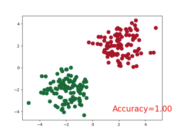
# 分类 Classification
import torch
import torch.nn.functional as F
from torch.autograd import Variable
import matplotlib.pyplot as plt

# 不同的代码
n_data = torch.ones(100, 2)
x0 = torch.normal(2 * n_data, 1)  # class0 x data (tensor), shape=(100, 2)
y0 = torch.zeros(100)  # class0 y data (tensor), shape=(100, 2)
x1 = torch.normal(-2 * n_data, 1)  # class1 x data (tensor), shape=(100, 2)
y1 = torch.ones(100)  # class2 y data (tensor), shape=(100, 2)
x = torch.cat((x0, x1), 0).type(torch.FloatTensor)  # FloatTensor = 32-bit floating
y = torch.cat((y0, y1), ).type(torch.LongTensor)  # LongTensor = 64-bit integer

x, y = Variable(x), Variable(y)

plt.scatter(x.data.numpy()[:, 0], x.data.numpy()[:, 1], c=y.data.numpy(), s=100, lw=0, cmap='RdYlGn')
plt.show()


# 打印
# plt.scatter(x.data.numpy(), y.data.numpy())
# plt.show()

class Net(torch.nn.Module):
    def __init__(self, n_feature, n_hidden, n_output):
        super(Net, self).__init__()
        self.hidden = torch.nn.Linear(n_feature, n_hidden)
        self.predict = torch.nn.Linear(n_hidden, n_output)

    def forward(self, x):
        x = F.relu(self.hidden(x))
        x = self.predict(x)
        return x


net = Net(2, 10, 2)
print(net)

plt.ion()
plt.show()

optimizer = torch.optim.SGD(net.parameters(), lr=0.02)
loss_func = torch.nn.CrossEntropyLoss()

for t in range(100):
    out = net(x)
    loss = loss_func(out, y)

    optimizer.zero_grad()
    loss.backward()
    optimizer.step()

    if t % 2 == 0:
        # plot and show learning process
        plt.cla()
        prediction = torch.max(F.softmax(out, dim=1), 1)[1]  # 预测分类结果
        pred_y = prediction.data.numpy()
        target_y = y.data.numpy()
        plt.scatter(x.data.numpy()[:, 0], x.data.numpy()[:, 1], c=pred_y, s=100, lw=0, cmap='RdYlGn')
        accuracy = float((pred_y == target_y).astype(int).sum()) / float(target_y.size)
        plt.text(1.5, -4, 'Accuracy=%.2f' % accuracy, fontdict={'size': 20, 'color': 'red'})
        plt.pause(0.1)

plt.ioff()
plt.show()

1
2
3
4
5
6
7
8
9
10
11
12
13
14
15
16
17
18
19
20
21
22
23
24
25
26
27
28
29
30
31
32
33
34
35
36
37
38
39
40
41
42
43
44
45
46
47
48
49
50
51
52
53
54
55
56
57
58
59
60
61
62
63
64
65
66
67
68

快速搭建神经网络

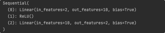
net2 = torch.nn.Sequential(
    torch.nn.Linear(2,10),
    torch.nn.ReLU(),
    torch.nn.Linear(10,2),
)
print(net2)

1
2
3
4
5
6

保存及提取

# 保存及提取神经网络
import torch
import matplotlib.pyplot as plt

# torch.manual_seed(1)    # reproducible

# fake data
x = torch.unsqueeze(torch.linspace(-1, 1, 100), dim=1)  # x data (tensor), shape=(100, 1)
y = x.pow(2) + 0.2*torch.rand(x.size())  # noisy y data (tensor), shape=(100, 1)

# The code below is deprecated in Pytorch 0.4. Now, autograd directly supports tensors
# x, y = Variable(x, requires_grad=False), Variable(y, requires_grad=False)


def save():
    # save net1
    net1 = torch.nn.Sequential(
        torch.nn.Linear(1, 10),
        torch.nn.ReLU(),
        torch.nn.Linear(10, 1)
    )
    optimizer = torch.optim.SGD(net1.parameters(), lr=0.5)
    loss_func = torch.nn.MSELoss()

    for t in range(100):
        prediction = net1(x)
        loss = loss_func(prediction, y)
        optimizer.zero_grad()
        loss.backward()
        optimizer.step()

    # plot result
    plt.figure(1, figsize=(10, 3))
    plt.subplot(131)
    plt.title('Net1')
    plt.scatter(x.data.numpy(), y.data.numpy())
    plt.plot(x.data.numpy(), prediction.data.numpy(), 'r-', lw=5)

    # 2 ways to save the net
    torch.save(net1, '04net.pkl')  # save entire net
    torch.save(net1.state_dict(), '04net_params.pkl')   # save only the parameters


def restore_net():
    # restore entire net1 to net2
    net2 = torch.load('04net.pkl')
    prediction = net2(x)

    # plot result
    plt.subplot(132)
    plt.title('Net2')
    plt.scatter(x.data.numpy(), y.data.numpy())
    plt.plot(x.data.numpy(), prediction.data.numpy(), 'r-', lw=5)


def restore_params():
    # restore only the parameters in net1 to net3
    net3 = torch.nn.Sequential(
        torch.nn.Linear(1, 10),
        torch.nn.ReLU(),
        torch.nn.Linear(10, 1)
    )

    # copy net1's parameters into net3
    net3.load_state_dict(torch.load('04net_params.pkl'))
    prediction = net3(x)

    # plot result
    plt.subplot(133)
    plt.title('Net3')
    plt.scatter(x.data.numpy(), y.data.numpy())
    plt.plot(x.data.numpy(), prediction.data.numpy(), 'r-', lw=5)
    plt.show()

# save net1
save()

# restore entire net (may slow)
restore_net()

# restore only the net parameters
restore_params()

1
2
3
4
5
6
7
8
9
10
11
12
13
14
15
16
17
18
19
20
21
22
23
24
25
26
27
28
29
30
31
32
33
34
35
36
37
38
39
40
41
42
43
44
45
46
47
48
49
50
51
52
53
54
55
56
57
58
59
60
61
62
63
64
65
66
67
68
69
70
71
72
73
74
75
76
77
78
79
80
81
82
83

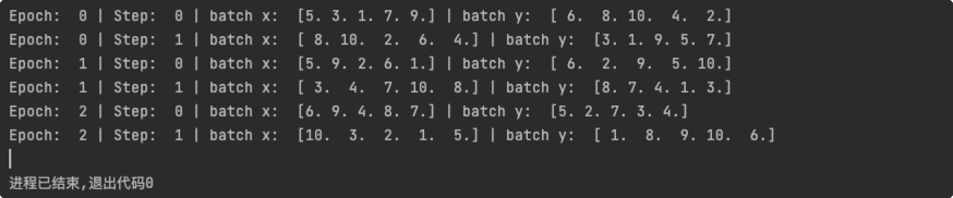
分批训练

# 分批训练
import torch
import torch.utils.data as Data

torch.manual_seed(1)    # reproducible

BATCH_SIZE = 5
# BATCH_SIZE = 8

x = torch.linspace(1, 10, 10)       # this is x data (torch tensor)
y = torch.linspace(10, 1, 10)       # this is y data (torch tensor)

torch_dataset = Data.TensorDataset(x, y)
loader = Data.DataLoader(
    dataset=torch_dataset,      # torch TensorDataset format
    batch_size=BATCH_SIZE,      # mini batch size
    shuffle=True,               # random shuffle for training
    num_workers=2,              # subprocesses for loading data
)


def show_batch():
    for epoch in range(3):   # train entire dataset 3 times
        for step, (batch_x, batch_y) in enumerate(loader):  # for each training step
            # train your data...
            print('Epoch: ', epoch, '| Step: ', step, '| batch x: ',
                  batch_x.numpy(), '| batch y: ', batch_y.numpy())


if __name__ == '__main__':
    show_batch()

1
2
3
4
5
6
7
8
9
10
11
12
13
14
15
16
17
18
19
20
21
22
23
24
25
26
27
28
29
30
31

人工智能（ArtificialIntelligence） #

资源链接 #

环境安装 #

！验证GPU加速 #

编辑器安装 #

激励函数 (Activation) #

回归 Regression #

分类 Classification #

快速搭建神经网络 #

保存及提取 #

分批训练 #